
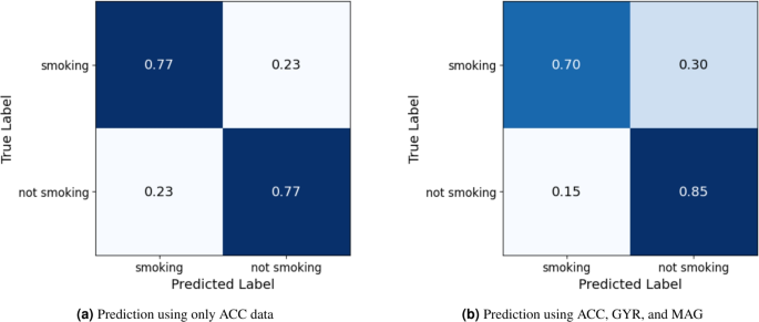
In order to develop an effective smoking-behaviour identification model, it was necessary to create a large dataset that includes smoking events, as reported in real time, alongside automatically collected data from the smokers’ smartphone sensors. This dataset can be made available upon request, adhering to ethical and commercialisation requirements. Using this dataset, the present study focused on the development of a DL model that could be trained to learn patterns within these data to predict smoking-related behaviour. The focus is exclusively on comparing advanced DL architectures, evaluating and comparing 1D-CNN, Long Short-Term Memory (LSTM), Bidirectional LSTM (BiLSTM), and hybrid combined models. This focus is driven by previous work, which demonstrated that DL approaches, particularly the 1D-CNN, outperformed traditional methods (such as Support Vector Machines: SVM and Decision Trees: DT models) in predicting smokers’ behaviour13.
Creation of dataset
Seventeen smokers (10 Females and 7 males, Mean age 37.18, minimum 5 cigarettes a day for at least 6 months) were recruited for the study and were financially compensated for their time. The study received full ethical approval from the Manchester Metropolitan University ethics committee. Before condensing and cleaning the data, the entire dataset included 404478 5-min samples. These were divided based on the two phases of data-collection Phase 1, pre-quitting, included 81837 5-minute samples, while Phase 2, post-quitting, included 322641 samples. The final data set (after pre-processing, see Sect. “Data processing” below) used for the training and validation process included a total of 2572 Phase 1 and 3616 Phase 2 5-minute data period samples (overall smoking lapses: 158, craving reporting: 1650, and 4337 non-smoking events).
Data were collected using a simple smartphone app. In Phase 1 of the data collection smokers were asked to report in real time, by pressing a button on their app, every cigarette they smoked over a two-week period. At the end of the two weeks, participants were given a 5-day window in which to quit smoking, before progressing to the Phase 2 of data collection. In Phase 2, participants were asked to report, over the three-month post-quitting period, any smoking lapses. They were also asked to report their craving level on a scale from 1 (very low) to 5 (very high), every time that they experienced high craving, or at least once a day if they did not experience high cravings (whenever they remembered to do so). This was important as a measure of engagement with the app. Smartphones’ sensor data (Accelerometer: ACC; Gyroscope: GYR; Magnetometer: MAG; Light: L; Time of the Day: T and GPS) were continuously recorded every minute throughout both phases of data collection.
Data processing
The collected data was pre-processed and then fed into four different DL models. Each model was assessed for its effectiveness in predicting smoking events during the pre-quit period (Phase 1) and instances of smoking lapses and cravings after quitting (Phase 2).
To develop a DL prediction model with a 5-minute prediction period, the collected data was converted to non-overlapped 5-minutes samples. This is common practice in action prediction ML models when training uses samples that are derived from raw signal data32,33. All data samples with a majority of missing samples were removed (as these are not useful for modelling), and the remaining samples were assigned either a (0) value for non-smoking samples or (1) for smoking events pre-quitting and reported cravings and lapses post quitting. Finally, to avoid the unbalanced data problem34, the data was randomly down sampled with noise removal35,36. Down sampling may be considered problematic in addiction research37 as the emphasis is on the ‘event’ (lapsing) rather than ‘non-event’ (non-smoking is a non-event); therefore additional results are reported which consider the non-sampled data (as processed through the current algorithm) in Appendix A. Each data sample included 25 rows of smartphone sensor data, with each row consisting of 5 columns (i.e. ACC, GYR, MAG, L, & T). GPS data was not used in the model, as due to the sensitivity of the data, modern smartphones only enable GPS data collection when the app is open. This corresponded with smokers reporting an event on the app, making the data highly biased as it was only available for smoking and craving samples.
The model can predict smoking events and cravings with high accuracy within a 5-min period. This represents enormous progress compared to previous work13. It is concluded that: (a) a combined 1D-CNN-BiLSTM is superior in computing temporal patterns of smoking behaviour, (b) combined accelerometers, gyroscopes, and magnetometers data give best predictions compared to each on their own, and compared to other predictors, and that (c) the model is capable of predicting the behaviour of new smokers, whose data was not used to train the DL model. The developed DL algorithm achieved 0.85 accuracy in predicting smoking behaviour before quitting and 0.77 accuracy in identifying high cravings and lapses post-quitting. This precision in predicting high-risk situations presents a promising opportunity for delivering timely interventions to support individuals during the quitting process. Despite some limitations, the findings underscore the promising role of smartphones’ sensors’ data and DL methods in advancing the understanding and intervention provision for smoking, and potentially other health behaviours, paving the way for more personalised and effective health interventions.
Deep learning model for smoking behaviour prediction
The research utilised a stacked DL model that combines 1D-CNN38 and BiLSTM39,40 units. In the combined DL model, the 1D-CNN component can learn local patterns from the input data but it cannot learn sequential correlations, whereas the BiLSTM component is specialised for sequential modelling, and can extract correlated patterns. Therefore, the combined model has the potential to improve the prediction accuracy of smoking (and craving) events, as this requires processing of large environmental datasets produced by phone sensors (input), while correlating it with smoking related events in the past and the (sequential correlations). This approach was shown to be effective in several domains, including time series prediction and health applications38,41,42.
The input layer accepts n-input vector (n is the number of inputs that changes based on the used data, ACC, GYR, MAG, T, & L) each with 25 rows of data (at 5 samples of data for each minute, 25 rows represents a total duration of 5 minutes). This is passed to the convolutional layer, with a filter size of 128; the convolutional operation takes the form
$$\begin{aligned} C_i=h(w^T\bigotimes x_{i-10:i}\ +b_i), \end{aligned}$$
(1)
where \(\bigotimes\) is convolution operator, \(w^T\) the network weights, b is the bias and h is a non-linear ReLU activation function with \(l_2\) weight regularisation. The feature map output of this layer is then batch normalised43, followed by a max-pooling layer that reduces the features’ variance,
$$\begin{aligned} P_{i,k}\ =\ Max\ (C_{(i,k)\ }U_{3,1}), \end{aligned}$$
(2)
where k is the filter number, and \(U_{3,1}\) is sliding max window of size (3 x 1).
The second stage of the DL model is the BiLSTM network43,44 (combining forward and backward LSTM models). Each LSTM consists of several multiplicative memory cells, each with three gates: input, output, and forget. These gates control the output from the cell, which is either ‘keep’, ‘release’, or ‘reset’; \(c_t\) denotes the cell state (memory state) at time step t, which carries long-term information through the sequence, and \(h_t\) denotes the hidden state at time step t, which represents the output of the LSTM cell and is passed to the subsequent layers.
$$\begin{aligned} f_t^\rightarrow= & \ \sigma \left( w_f^\rightarrow \cdot \left[ h_{t-1}^\rightarrow ,\ x_t^\rightarrow \right] +b_t^\rightarrow \right), \end{aligned}$$
(3)
$$\begin{aligned} i_t^\rightarrow= & \ \sigma \left( w_i^\rightarrow \cdot \left[ h_{t-1}^\rightarrow ,\ x_t^\rightarrow \right] +b_i^\rightarrow \right), \end{aligned}$$
(4)
$$\begin{aligned} {\widetilde{c}}_t^\rightarrow= & \ tanh{\left( w_c^\rightarrow \cdot \left[ h_{t-1}^\rightarrow ,\ x_t^\rightarrow \right] +b_c^\rightarrow \right), } \end{aligned}$$
(5)
$$\begin{aligned} c_t^\rightarrow= & \ f_t^\rightarrow *{\widetilde{c}}_{t-1}^\rightarrow +i_t^\rightarrow *{\widetilde{c}}_t^\rightarrow, \end{aligned}$$
(6)
$$\begin{aligned} o_t^\rightarrow= & \ \sigma \left( w_o^\rightarrow \cdot \left[ h_{t-1}^\rightarrow ,\ x_t^\rightarrow \right] +b_o^\rightarrow \right), \end{aligned}$$
(7)
$$\begin{aligned} h_t^\rightarrow= & \ o_t^\rightarrow *t a n h{\left( c_t^\rightarrow \right) }. \end{aligned}$$
(8)
In the BiLSTM \(f_i\), \(i_t\), and \(o_t\) are calculated for both forward and backward networks; \(h_t^\rightarrow\) for the forward LSTM network is calculated using the current t and the previous \(t-1\) instances, While the \(h_t^\leftarrow\) for the backward LSTM network is calculated using the current t and the next \(t+1\) as
$$\begin{aligned} f_t^\leftarrow= & \ \sigma \left( W_f^\leftarrow \cdot \left[ h_{t+1}^\leftarrow ,\ X_t^\leftarrow \right] +b_t^\leftarrow \right), \end{aligned}$$
(9)
$$\begin{aligned} i_t^\leftarrow= & \ \sigma \left( W_i^\leftarrow \cdot \left[ h_{t+1}^\leftarrow ,\ X_t^\leftarrow \right] +b_i^\leftarrow \right), \end{aligned}$$
(10)
$$\begin{aligned} {\widetilde{c}}_t^\leftarrow= & \ tanh{\left( W_c^\leftarrow \cdot \left[ h_{t+1}^\leftarrow ,\ X_t^\leftarrow \right] +b_c^\leftarrow \right) }, \end{aligned}$$
(11)
$$\begin{aligned} c_t^\leftarrow= & \ f_t^\leftarrow *{\widetilde{c}}_{t+1}^\leftarrow +i_t^\leftarrow *{\widetilde{c}}_t^\leftarrow, \end{aligned}$$
(12)
$$\begin{aligned} o_t^\leftarrow= & \ \sigma \left( W_o^\leftarrow \cdot \left[ h_{t+1}^\leftarrow ,\ X_t^\leftarrow \right] +b_o^\leftarrow \right), \end{aligned}$$
(13)
$$\begin{aligned} h_t^\leftarrow= & \ o_t^\leftarrow *t a n h{\left( c_t^\leftarrow \right) }. \end{aligned}$$
(14)
The final \(h_t\) is the concatenated vector of both \(h_t^\rightarrow\) and \(h_t^\leftarrow\),
$$\begin{aligned} h_t\ =[h_t^\rightarrow \ h_t^\leftarrow ]. \end{aligned}$$
(15)
The output from the BiLSTM is then passed to the final level of the model, which is made of three layers of a fully connected neural network. Specifically, the concatenated hidden state \(h_t\) is used as the input to the first dense layer. These are used to generate a binary output that represents a prediction of either a smoking or a non-smoking session in a 5-minute slot.
